Analysis of AX discrimination data
1. AX design,
stimuli drawn in pairs from along a continuum
AX: a pair of stimuli; is X the same as A, or different?;
response = "same" or "different" .
roving (vs fixed): the A stimulus varies along the continuum
just as the X does, rather than serving as a fixed standard
ISI: InterStimulus Interval, time between the
stimuli in a pair. The longer the ISI, the more likely the response
will reflect a categorization of the stimuli. Half a second is plenty
of time for a subject to give a response.
same trials: for some of the trials, the stimuli will be identical.
A difficult design question is what proportion of trials should be same
trials. Many different trials will sound the same to listeners,
so if half the trials are same trials, most of the responses will be
"same", which is boring and/or alarming for subjects.
step size: the distance between the stimuli in a pair, in
terms of steps along the continuum. 1-step: adjacent on the continuum.
Obviously the step-size per se has no importance, as it depends on how the
continuum was constructed (e.g. a 2-step pair from a 5 msec VOT continuum
is the same as a 1-step pair from a 10 msec VOT continuum); but for a given
continuum larger steps are easier to discriminate.
Discrimination experiments last longer than
the corresponding identification experiments. Although there are fewer
different pairs than there are singleton stimuli, there are same
pairs as well, and each trial is longer (2 stimuli + ISI).
2. Tabulating responses
Much as for identification responses, discrimination
responses can be tabulated as the proportion of the repetitions of a pair
classified as "same" or as "different". Unlike identification responses,
discrimination responses are right or wrong, so they can also be tabulated
as the proportion of the repetitions judged correctly. (For the different
trials, these 2 measures are the same, and often the same trials are
not tabulated at all.) Depending on the response bias of a listener,
trials heard as "same" might be judged anywhere from 0% different (listener
is tends to respond "same") to 50% different (listener responds at chance).
Graphing: The x-axis is the stimulus dimension,
and by convention the value of a pair of stimuli is taken to be the mid-point
between the values of the 2 stimuli. E.g. the x-value of a pair (+10,
+20) is +15, while the x-value of a pair (+10, +30) is +20.
practice file: discrim_data.xls,
sheet 1: pretend data
from a VOT continuum, values are proportion "different" out of 10 repetitions.
How to analyze?
3. ANOVA, just
as for identification data
By itself a 1-way ANOVA on stimulus pair
will tell you if subjects treated the pairs differently (which they virtually
always do); more interesting will be post-hoc tests/planned comparisons.
Such tests will tell you which stimulus pairs are perceived differently from
which others, and this is a relevant research question for discrimination
data.
practice file: discrim_data.xls,
sheet 2: ready to open in SPSS
· one continuum, 2 groups of subjects (sheet 2)
· same data, but now from 1 group of subjects, comparing
across continua (sheet 3) (if you enter the factors in the order pair(7),
continuum(2), you can practice matching factor levels to variable columns
by hand)
4. Fit a curve/function to the
responses? No, never seen.
5. Analysis of the discrimination
peak (across continua and/or subject
groups)
Discrimination peak: well-discriminated
pair(s), usually with higher responses than to other pairs, thus forming a
peak in the plotted discrimination responses.
location: which pair along the continuum is discriminated
the best?
height: what is the greatest proportion of responses?
width (not generally quantified): how many pairs are
discriminated well, e.g. above chance? This is a measure made up for
this exercise, but a sensible one.
practice file: discrim_data.xls,
sheet 1 right columns, and last sheet
(above chance
here = 8/10 or better, by a binomial test)
6. Relating discrimination responses
to identification responses: within- vs. across-category pairs
The discrimination peak is expected to span
the identification boundary. That is, expectations about performance
are different for different pairs drawn from within a single phonetic/phonemic
category, vs. from 2 different categories. Since such a classification
of the pairs as within vs. across categories can be established a priori,
planned comparisons are appropriate. (Really, the classification should
be established for each individual subject from that subject's identification
responses. But it is generally established for the group as a whole;
and in one study of normal and dyslexic children, published adult identification
data were used to establish the within and across pairs for the child subjects.)
Or, often the responses to all within-category pairs are averaged, and likewise
to all across-category pairs, and these averages are compared (e.g. by paired
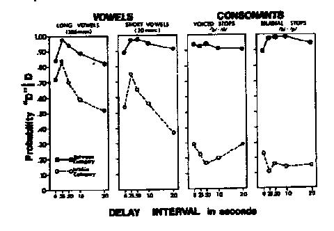
t-test). Here is an example (p. 256) from Pisoni (1973), Perc. & Psychophys. 13(2): 253-260,
in which the x-axis variable is ISI.
The filled datapoints are means of across-category pairs, and the open
datapoints are means of within-category pairs, for 4 different continua.
Relating discrimination responses to
identification responses: comparing predicted vs. obtained discrimination
7. Let's look at the relation between
some pretend ID and discrimination data, checking out the locations of the
categories and, qualitatively, the correspondence between the 2 sets of data.
Recall that categorical perception refers to perception by categories, specifically,
discrimination limited by categorization.
practice file: discrim_ID_data.xls,
top sheet right columns
In the ideal case, identification will be
perfectly categorical (abrupt boundary between 2 adjacent stimuli).
The discrimination peak should cross this 1-step category boundary, and all
other pairs should be discriminated at or below chance. That is, if
a pair of stimuli (a,b) have opposite categorizations (0,1 or 1,0) then their
discrimination score will be 1, while if a pair of stimuli (a,b) have the
same categorization (0,0 or 1,1) then their discrimination score will be 0
(or at chance, depending on response bias).
Haskins researchers (originally, Liberman
et al. 1957, for ABX discrimination; see also Pollack
& Pisoni 1971, Psych. Sci.) predict
the discrimination score for a pair of stimuli, using the identification
score of each stimulus. With this formula, whenever the identification
of the 2 stimuli is the same - both 0, or
both .5, or any other value - the predicted discrimination is at chance. Here
is a general formula for AX discrimination data, taken from Godfrey et al.
(1981).
Predicted discrimination = (P1a
x P2b) + (P1b x P2a), where
·
P1a = proportion of times stimulus 1 was identified as
“a”
·
P2b = proportion of times stimulus 2 was identified as
“b”
·
P1b = proportion of times stimulus 1 was identified as
“b”
·
P2a = proportion of times stimulus 2 was identified as
“a”
Not surprisingly, this is not what real
discrimination data usually look like. (If identification of a stimulus
is split between the 2 responses, then discrimination of pairs including that
stimulus will be above chance; furthermore, even when the identification is
consistent, discrimination can still be above chance, because it can be based
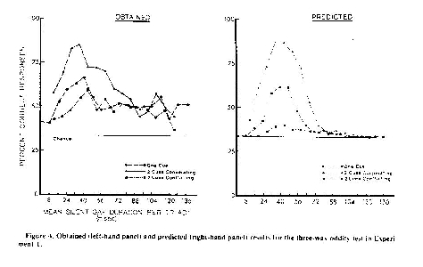
on auditory memory for the particular stimuli.) Here is an example from
Best et al. (1981), a rare paper in showing these predicted-discrimination
functions:
8. The relation between obtained and
predicted discrimination is then generally tested by ANOVA, with factors "obtained
vs. predicted" and "stimulus pairs". The typical result is that both
factors, and their interaction, are significant. That is, the obtained
and predicted functions are different, but only for certain pairs - the within-category
pairs, which are discriminated better than predicted. (The across-category
pairs are generally discriminated perfectly, as predicted.) This result
- better obtained than predicted discrimination - goes back to the first
paper to present this kind of analysis, Liberman et al. (1957).
Prepared by Pat Keating, Spring 2004